pacman::p_load(tidyverse, ggrepel, patchwork,
               ggthemes, hrbrthemes,
tidyverse, ggdist, ggridges, colorspace,gridExtra)take home exercise 3
Background
As we know Singapore is situated near the equator and it has a typically tropical climate. It has 2 two monsoon seasons, one is Northeast Monsoon(December to early March); the other is Southwest Monsoon(une to September). In this task, we will choose December to analysis the temperature variation.
Purpose
Daily mean temperatures are projected to increase by 1.4°C to 4.6°C, while annual mean temperatures rose at an average rate of 0.25°C per decade. We want to find out the reasons.
Import data
I choose the Changi station, December 1983, 1993, 2003, 2013, 2023’ temperature data by grouping the data manually. R can not read the degree, so I moved it out.
TEMData <- read_csv("data/DEC1983-2023TEM.csv") glimpse(TEMData)Rows: 155
Columns: 10
$ Station <chr> "Changi", "Changi", "Changi", "Changi", "C…
$ Year <dbl> 1983, 1983, 1983, 1983, 1983, 1983, 1983, …
$ Month <dbl> 12, 12, 12, 12, 12, 12, 12, 12, 12, 12, 12…
$ Day <dbl> 1, 2, 3, 4, 5, 6, 7, 8, 9, 10, 11, 12, 13,…
$ `Daily Rainfall Total (mm)` <dbl> 2.8, 1.7, 5.0, 8.2, 0.0, 0.0, 0.0, 19.8, 4…
$ `Mean Temperature` <dbl> 26.4, 24.3, 25.1, 25.2, 26.0, 25.0, 25.6, …
$ `Maximum Temperature` <dbl> 31.0, 27.2, 30.2, 30.3, 29.8, 27.7, 28.8, …
$ `Minimum Temperature` <dbl> 23.8, 21.9, 23.2, 23.0, 23.0, 23.7, 23.4, …
$ `Mean Wind Speed (km/h)` <dbl> 9.1, 4.9, 3.1, 3.2, 4.5, 4.4, 4.9, 5.4, 6.…
$ `Max Wind Speed (km/h)` <dbl> 46.1, 36.4, 41.0, 31.7, 28.8, 32.4, 32.8, …Data description & Process of thinking.
Ridgeline plot(also known as Joyplot) is a method to display the distribution of a numeric value for several groups. We use this method to display the December of 1983, 1993, 2003, 2013, 2023’s daily mean temperature.
ggplot(data = TEMData,
       aes(x = `Mean Temperature`, y = as.factor(Year),
           fill = after_stat(x))) +
    geom_density_ridges_gradient(
    scale = 3,
    rel_min_height = 0.01) +
  scale_fill_viridis_c(name = "Temp (°C)",
                       option = "C") +
  scale_x_continuous(
    name = "Mean Temperature",
    expand = c(0, 0)
  ) +
  scale_y_discrete(
    expand = expansion(add = c(0.2, 2.6))
  ) +
  theme_ridges() +
  labs(title = "Dec Temperature Distribution by Year",
    y = "Year")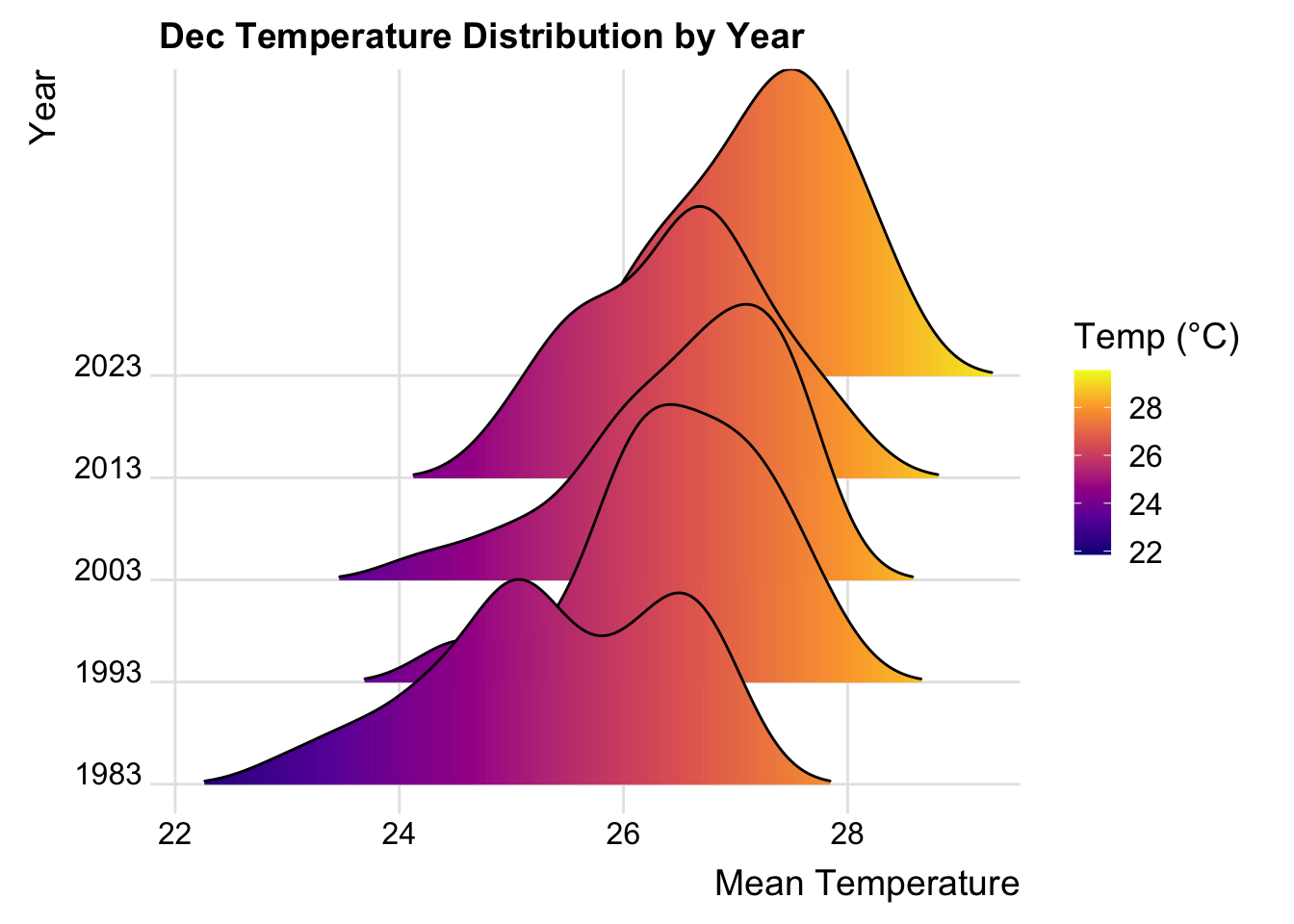
ggplot(TEMData,
       aes(x = `Mean Temperature`, y = as.factor(Year),
           fill = 0.5 - abs(0.5-stat(ecdf)))) +
  stat_density_ridges(geom = "density_ridges_gradient",
                      calc_ecdf = TRUE) +
  scale_fill_viridis_c(name = "Tail probability",
                       direction = -1) +
  theme_ridges()+
  labs(title = "Dec Temperature Distribution by Year",
    y = "Year")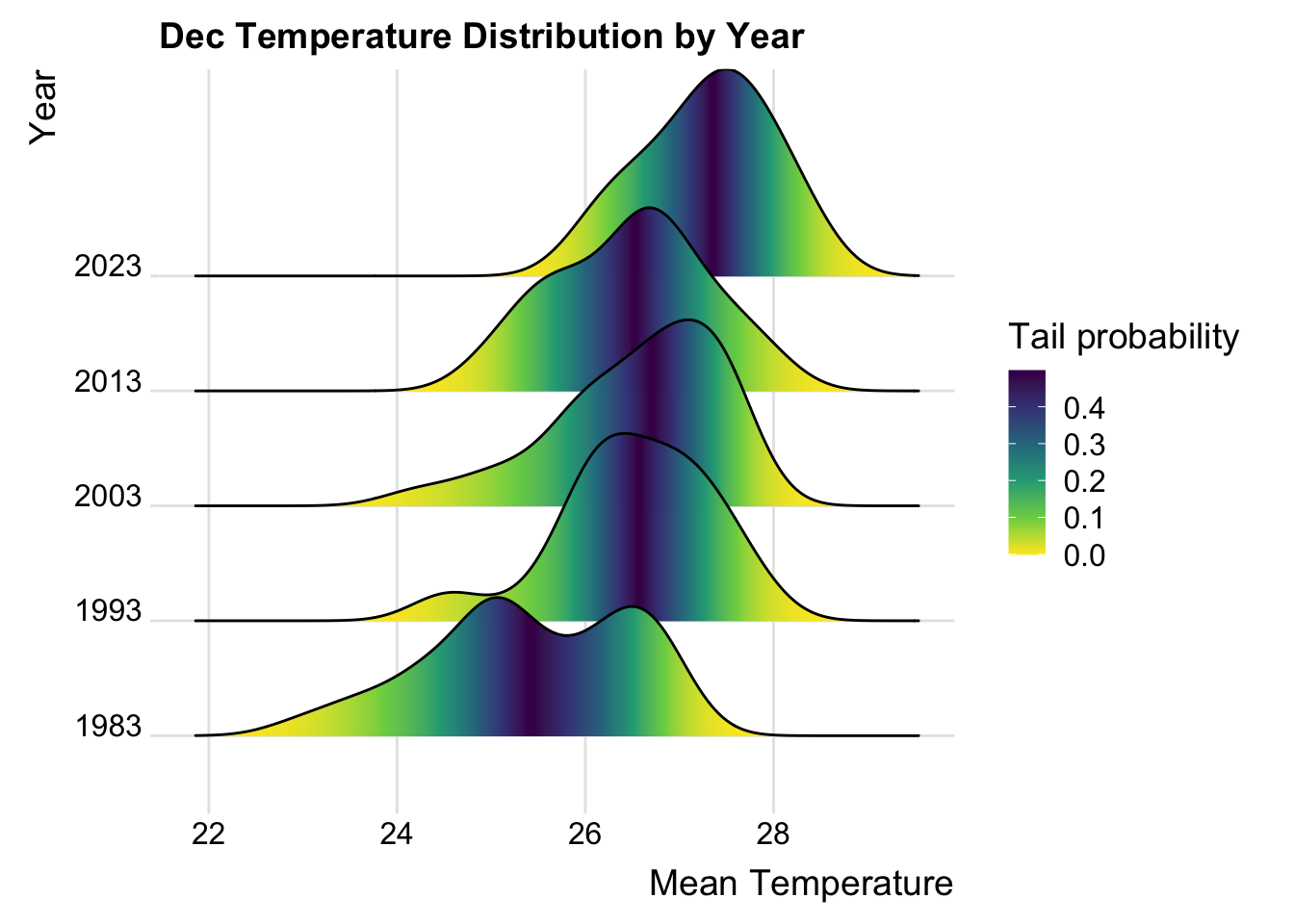
ggplot(TEMData,
       aes(x = `Mean Temperature`, y = as.factor(Year),
           fill = factor(stat(quantile))
           )) +
  stat_density_ridges(
    geom = "density_ridges_gradient",
    calc_ecdf = TRUE,
    quantiles = 4,
    quantile_lines = TRUE) +
  scale_fill_viridis_d(name = "Quartiles") +
  theme_ridges() +
  labs(title = "Dec Temperature Distribution by Year",
    y = "Year")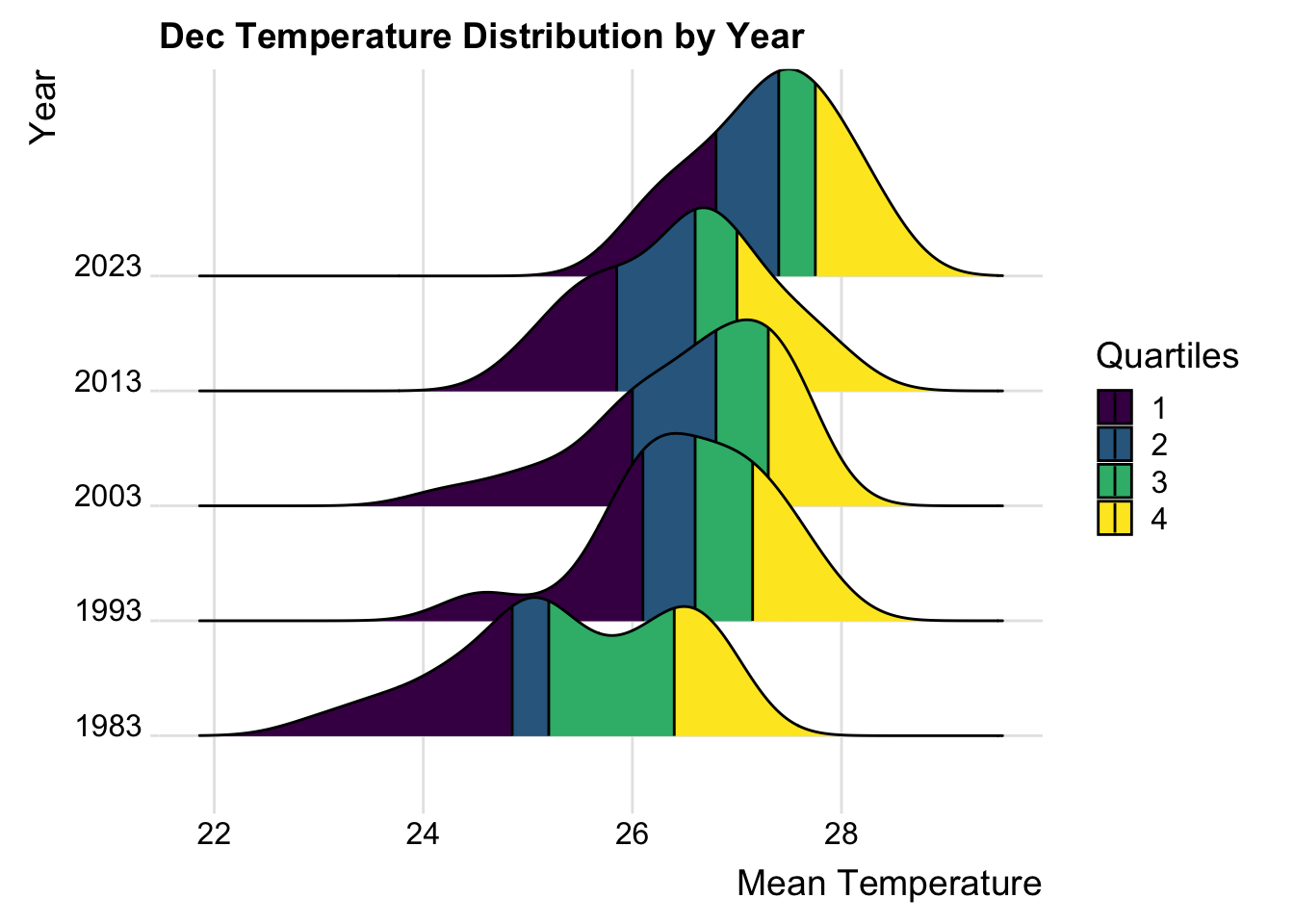
ggplot(TEMData,
       aes(x = `Mean Temperature`, y = as.factor(Year),
           fill = factor(stat(quantile))
           )) +
  stat_density_ridges(
    geom = "density_ridges_gradient",
    calc_ecdf = TRUE,
    quantiles = c(0.025, 0.975)
    ) +
  scale_fill_manual(
    name = "Probability",
    values = c("#FF0000A0", "#A0A0A0A0", "#0000FFA0"),
    labels = c("(0, 0.025]", "(0.025, 0.975]", "(0.975, 1]")
  ) +
  theme_ridges()+
  labs(title = "Dec Temperature Distribution by Year",
    y = "Year")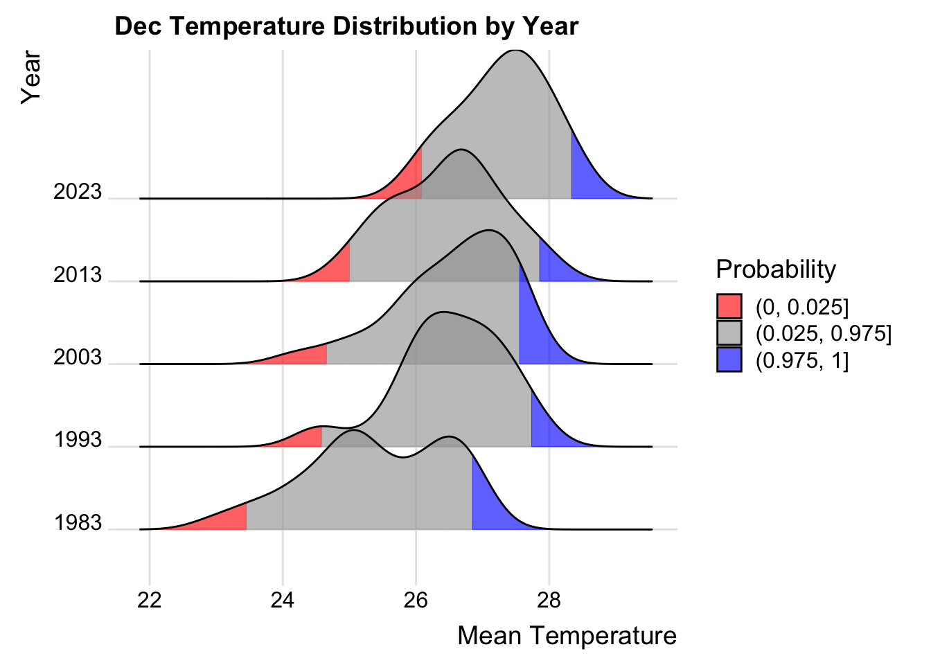
ggplot(TEMData,
       aes(x = as.factor(Year), y = `Mean Temperature`)) +
  stat_halfeye(adjust = 0.5,
               justification = -0.2,
               .width = 0,
               point_colour = NA) +
  labs(title = "Dec Temperature Distribution by Year",
    x = "Year")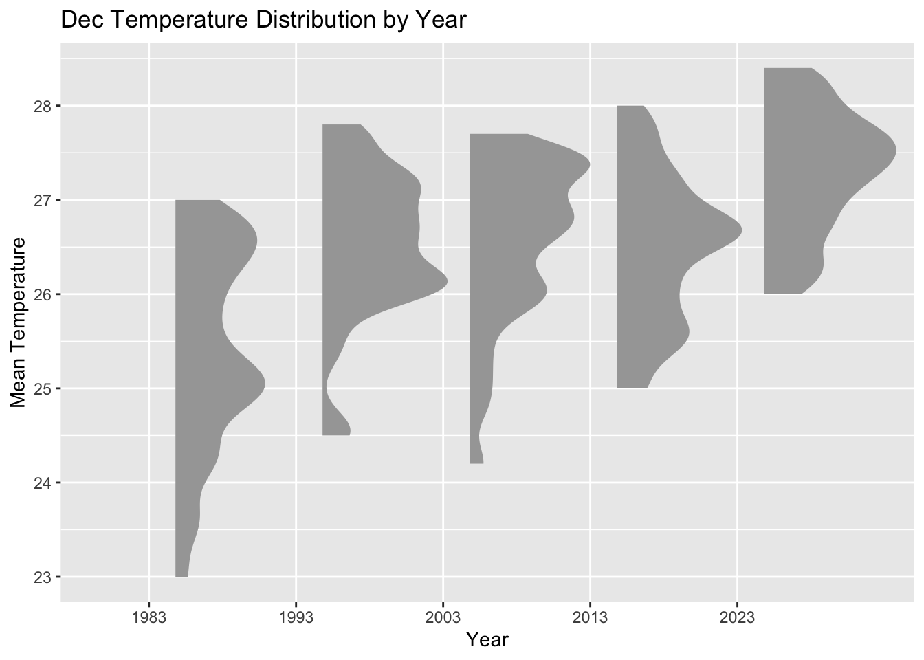
ggplot(TEMData,
       aes(x = as.factor(Year), y = `Mean Temperature`)) +
  stat_halfeye(adjust = 0.5,
               justification = -0.2,
               .width = 0,
               point_colour = NA) +
  geom_boxplot(width = .20,
               outlier.shape = NA) +
  labs(title = "Dec Temperature Distribution by Year",
    x = "Year")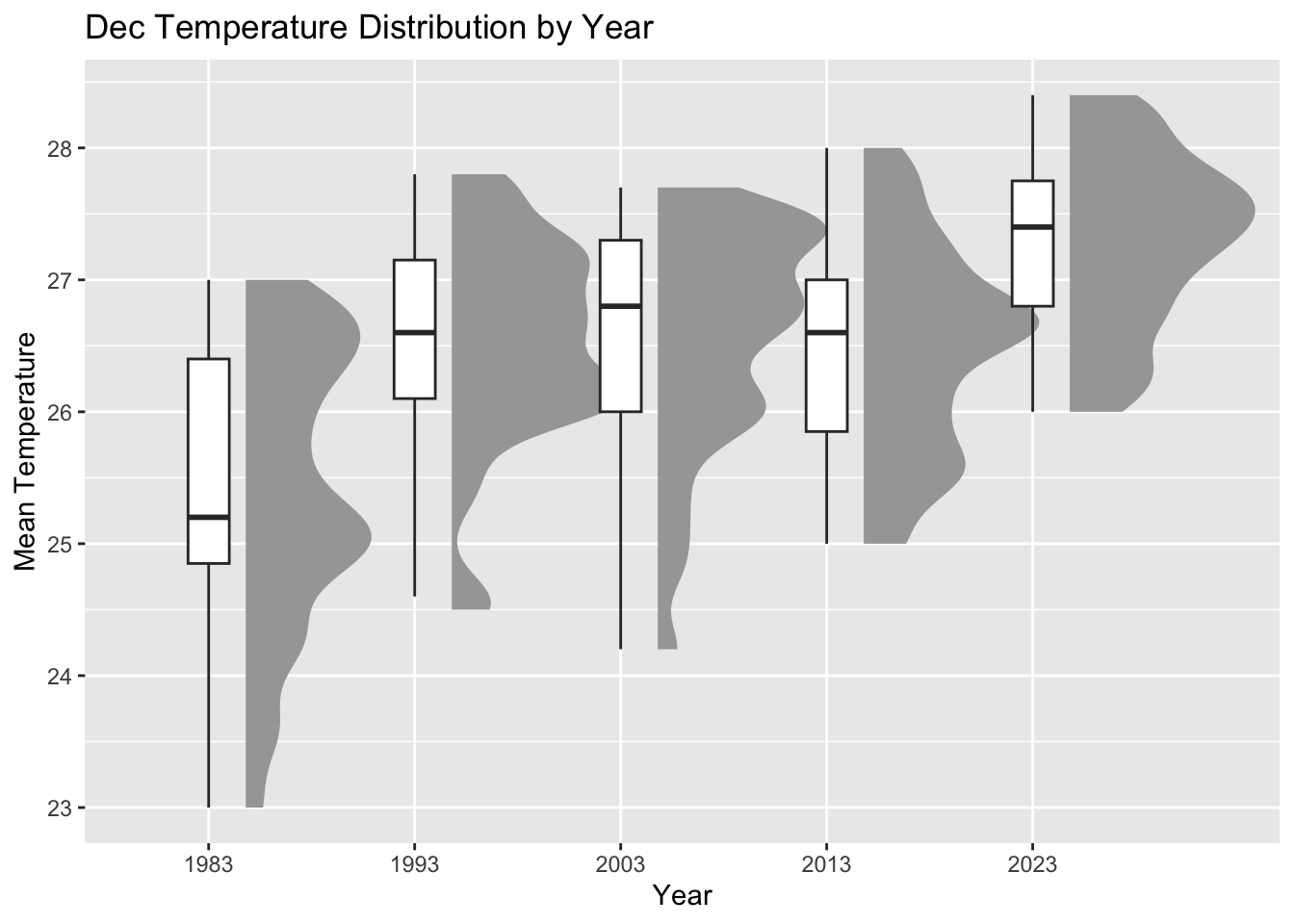
TEMData_means <- TEMData %>%
  group_by(Year) %>%
  summarise(MeanTemp = mean(`Mean Temperature`, na.rm = TRUE)) %>%
ungroup()ggplot(TEMData,
aes(x = as.factor(Year), y = `Mean Temperature`)) +
stat_halfeye(adjust = 0.5,
justification = -0.2,
.width = 0,
point_colour = NA) +
geom_boxplot(width = .20,
outlier.shape = NA) +
stat_dots(side = "left",
justification = 1.2,
binwidth = .5,
dotsize = 0.1)+
labs(title = "Dec Temperature Distribution by Year",
x = "Year") +
geom_text(data = TEMData_means, aes(label = round(MeanTemp, 1), y = MeanTemp),
nudge_x = 0.25, hjust = 0, check_overlap = TRUE)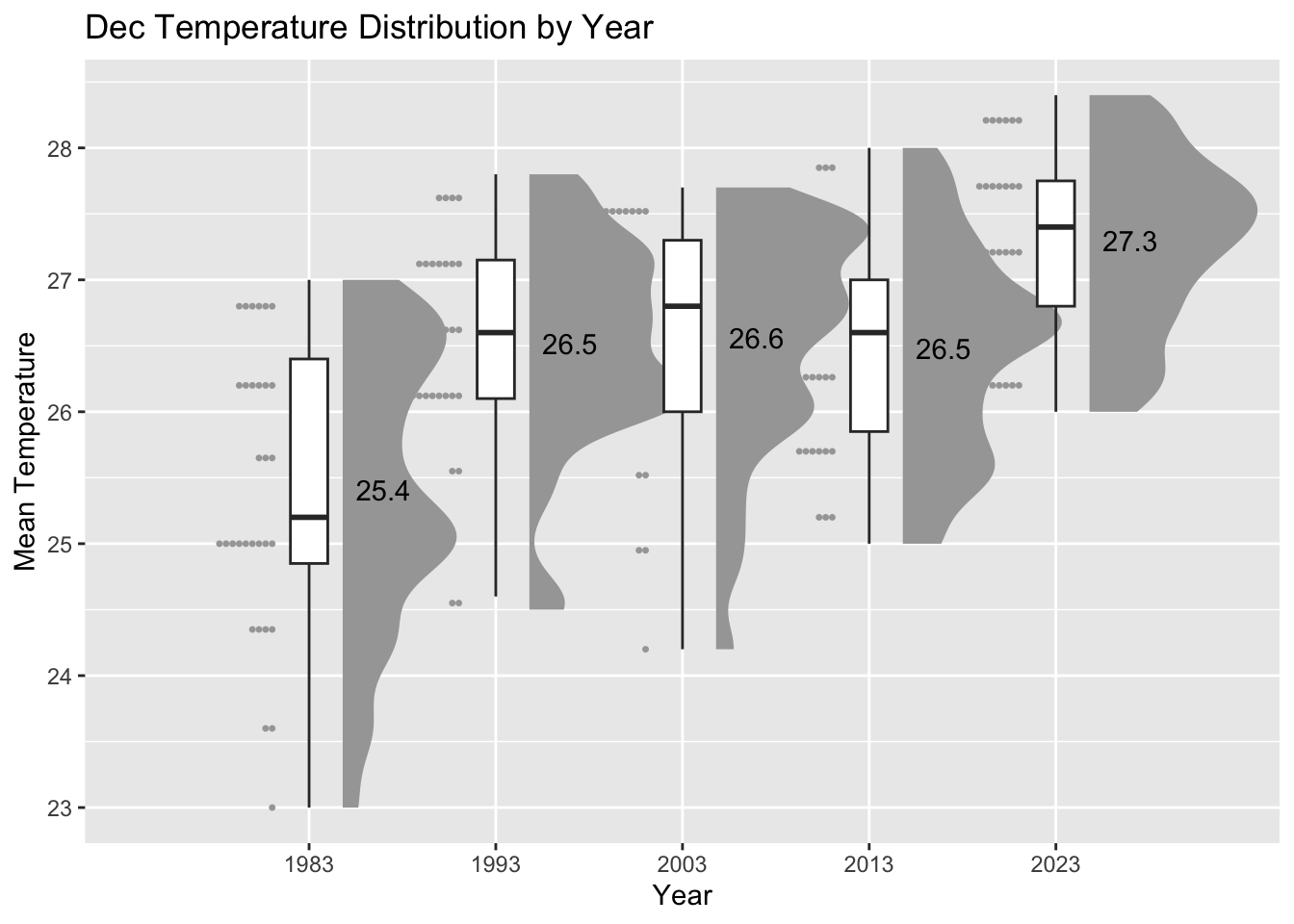
Final result
TEMData_max <- aggregate(`Mean Temperature` ~ Year, data = TEMData, max)
TEMData_min <- aggregate(`Mean Temperature` ~ Year, data = TEMData, min)
p1 <-ggplot(TEMData, aes(x = as.factor(Year), y = `Mean Temperature`)) +
labs(y = "Mean Temperature (°C)", x = "Year") +
stat_halfeye(adjust = 0.5,
justification = -0.2,
.width = 0,
point_colour = NA) +
geom_boxplot(width = .20,
outlier.shape = NA) +
stat_dots(side = "left",
justification = 1.2,
binwidth = .5,
dotsize = 0.1) +
coord_flip() +
theme_economist() +
labs(title = "Dec Temperature Distribution by Year",
x = "Year") +
geom_text(data = TEMData_means, aes(label = round(MeanTemp, 1), y = MeanTemp),
nudge_x = 0.25, hjust = 0, check_overlap = TRUE) +
geom_text(data = TEMData_max, aes(label = `Mean Temperature`, y = `Mean Temperature`),
nudge_x = 0.25,nudge_y = -0.25, hjust = 0, check_overlap = TRUE) +
geom_text(data = TEMData_min, aes(label = `Mean Temperature`, y = `Mean Temperature`),
nudge_x = 0.25, hjust = 0, check_overlap = TRUE) TEMData_diff <- data.frame(
Year = TEMData_max$Year,
Diff = TEMData_max$`Mean Temperature` - TEMData_min$`Mean Temperature`
)p2 <- ggplot(TEMData_diff, aes(x = as.factor(Year), y = Diff)) +
geom_bar(stat = "identity", fill = "grey")+
geom_text(aes(label = Diff), position = position_dodge(width = 0.9), hjust = 0.8) +
coord_flip() +
theme_economist() +
labs(x = "", y = "Tem Diff (°C)")combined_plot <- p1 + p2 + plot_layout(widths =c(3, 1))
combined_plot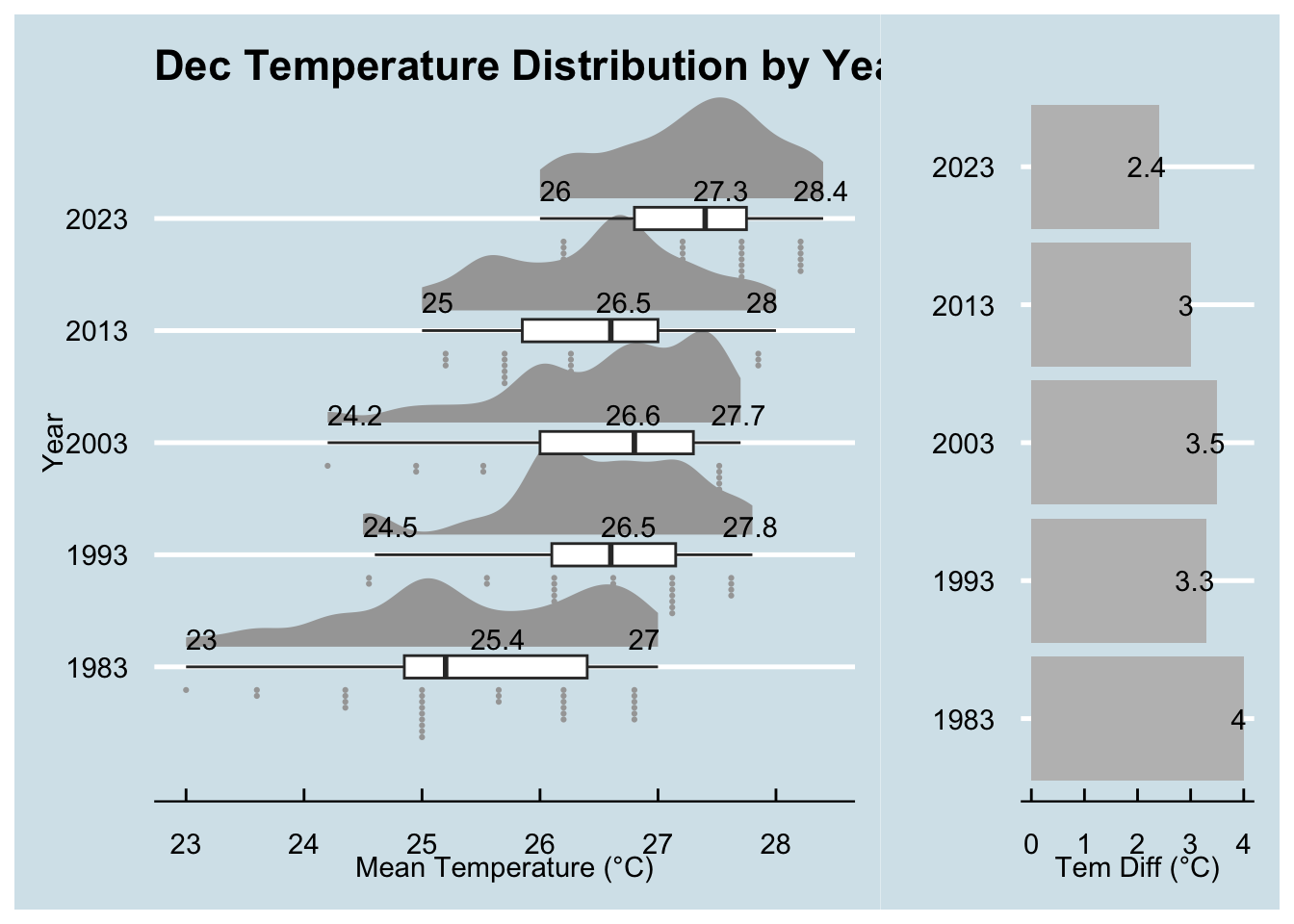
Summary
For this purpose, we want to find out the daily mean temperatures increase by 1.4°C to 4.6°C, while annual mean temperatures rose at an average rate of 0.25°C per decade.
In the chart, you can see the minimal daily mean temperature increase from 25.4°C to 27.3°C from December 1983 to 2023. The trend of minimal daily mean temperature increase from 23°C to 26°C, while the maximal daily mean temperature from 27°C to 28.4°C from the left chart. From the right chart, you can see the daily mean temperature narrow form 4°C to 2.4°C. So we can conclude that the temperature is rising, and the daily temperature range is decreasing, with the rate of change accelerating.